Changepoint analysis using Stan
A chart from The Atlantic has made the rounds, going viral on Twitter.

Naturally, everyone has their own interpretation of what it means and what trends the data shows. Here’s Derek Thompson:
Holy crap this thing went bonkers viral.
— Derek Thompson (@DKThomp) February 29, 2024
So, one way to see this data is to break down the decline
Total 1976-2022 hangout decline for girls is -30%pts
- 1976-2000 change: -4 %pts
- 2000-'12: -9%pts
- 2012-'22 : -17 %pts
So ya, something happened in that last decade. https://t.co/c5eJfh1N3n
Rather than eyeball it, I think a more principled approach is to let the data speak. Okay, you got me: we always bring in our own assumptions and the data never “speaks for itself”. But this chart does give me an excuse to run a changepoint model. Why? Because I feel like it.
Reproducing the chart
Our first step is to reproduce the chart. The data for the chart comes from Monitoring the Future, a well-run survey of American 8th, 10th, and 12th graders. The data is publicly available, so we can download it. It’s a bit of pain to download, and I could not find a way in R to do so in a reproducible way. So if you want to run the script below, you’ll need to download the relevant years of the survey, unzip it, and save the data from the core module in a folder (I saved them in a folder called “Data”). Assuming you did not change the file names, the script below should open them for you.
You can find the full script in the folder here
library(tidyverse)
library(haven)
library(survey)
library(here)
library(cmdstanr)
library(posterior)
library(bayesplot)
library(ThemePark)
library(tidybayes)

# Get a list of files
files_to_open <- list.files(paste0(here(), "/Data"))

# Read files into a list.
# Variables are not consistently named across years
d_list <- list()
for(i in 1:length(files_to_open)){
  d_list[[i]] <- read_dta(paste0(here(), "/Data/", files_to_open[i]))
}

# We need to extract variables of interest
# Because variables are inconsistently named, we'll need to recode them
# I'd like this part to be clearer, but sadly it isn't
# It will work fine so long as you didn't rename the files
recode_indicator <- c(rep(1, 10), 2, rep(1, 9), rep(3, 11))
data_to_combine <- list()
for(i in 1:length(files_to_open)){
  if(recode_indicator[i] == 1){
    data_to_combine[[i]] <- d_list[[i]][,c("V1", "V5", "V150", "V194")]
  } else if(recode_indicator[i] == 2){
    data_to_combine[[i]] <- d_list[[i]][, c("V5", "V8", "V13", "V58")]
  } else if(recode_indicator[i] == 3){
    data_to_combine[[i]] <- d_list[[i]][,c("V1", "ARCHIVE_WT", "V2150", "V2194")]
    }

  names(data_to_combine[[i]]) <- c("year", "WT", "Sex", "Wk_out")
}


# Combine data into one master file
d <- data_to_combine[[1]]

# Just turn the variables to numeric for now.
d$year <- as.numeric(d$year)
d$WT <- as.numeric(d$WT)
d$Wk_out <- as.numeric(d$Wk_out)
d$Sex <- as.numeric(d$Sex)

for(i in 2:length(data_to_combine)){
  d_tmp <- data_to_combine[[i]]

  d_tmp$year <- as.numeric(d_tmp$year)
  d_tmp$WT <- as.numeric(d_tmp$WT)
  d_tmp$Wk_out <- as.numeric(d_tmp$Wk_out)
  d_tmp$Sex <- as.numeric(d_tmp$Sex)

  d <- rbind(d, d_tmp)
}

# recode variables to produce the chart
d$Wk_out_cat <- ifelse(d$Wk_out %in% c(3, 4, 5, 6), "2 or more times a week", "< 2 times a week")
d$Wk_out_cat <- as.factor(ifelse(d$Wk_out %in% c(0, 9, -9), NA, d$Wk_out_cat))
d$Sex_cat <- ifelse(d$Sex == 1, "Male", "Female")
d$Sex_cat <- as.factor(ifelse(d$Sex %in% c(3, 4), "Other", d$Sex_cat))
d$Sex_cat[d$Sex == -9] <- NA
d$year <- ifelse(d$year < 100, d$year + 1900, d$year)


# Make survey design object to use weights
d_svy <- svydesign(ids = ~0, data = d, weights = d$WT)
d_agg <- svyby(~Wk_out_cat, ~year + Sex_cat, design = d_svy, FUN = svymean, na.rm = TRUE)
d_agg$twice_or_more <- d_agg$`Wk_out_cat2 or more times a week`
d_agg$se_twice_or_more <- d_agg$`se.Wk_out_cat2 or more times a week`
The chart
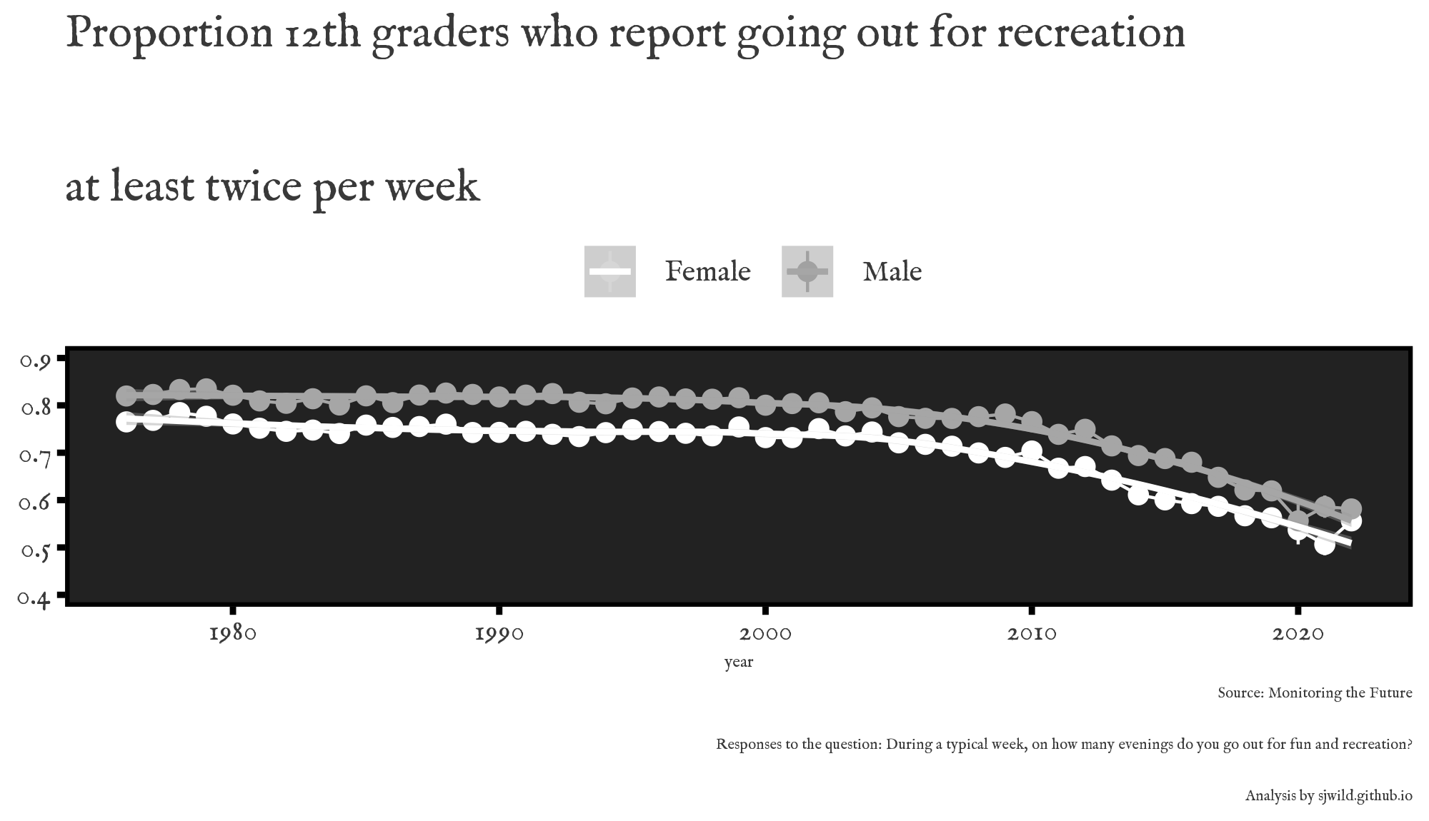
And with that, we can reproduce our chart. Because this is a fun post, let’s make use of the {ThemePark} package.
modified_theme_oppenheimer <- theme_oppenheimer() +
  theme(legend.direction = "horizontal",
        legend.position = "top",
        legend.background = element_rect(fill = "white"),
        plot.title = element_text(size = 48),
        axis.text = element_text(size = 30),
        legend.text = element_text(size = 30))

ggplot(subset(d_agg, Sex_cat != "Other"),
       mapping = aes(x = year,
                     y = twice_or_more,
                     group = Sex_cat,
                     colour = Sex_cat,
                     ymin = twice_or_more - 2 * se_twice_or_more,
                     ymax = twice_or_more + 2 * se_twice_or_more)) +
  geom_line() +
  geom_pointrange() +
  geom_smooth() +
  ylim(.4, .9) +
  labs(y = NULL,
       title = "Proportion 12th graders who report going out for recreation\nat least twice per week") +
  scale_colour_manual(values = c("white",
                                 "grey65"),
                      name = NULL) +
  labs(caption = "Source: Monitoring the Future\nResponses to the question: During a typical week, on how many evenings do you go out for fun and recreation?") +
  modified_theme_oppenheimer

ggsave("atlantic_recreation_reproduced.png", width = 2000, height = 1150, units = "px")

A changepoint model
As you can see from the plot, it looks like the trend starts around 2010. But who knows for sure. This is a yearly survey measuring something that likely changes during the course of the year. But that’s the subject for a future post.
For our purposes, we’re going to use a changepoint model, which allows us to identify a point in our time series during which our parameter of interest shifts, either heading higher or lower. We are essentially estimating two parameters: one for the first part and another for the second part. We are interested in estimating the point at which the parameter changes.
I can’t do a better job explaining it than do Wikipedia and the Stan manual, so head there and have read.
Stan code
The model in the Stan manual can easily be modified to account for different likelihoods. In our case, we’ll assume that we can model the yearly proportion of 12th graders reporting going out at least twice a week as coming from a normal distribution. There are definitely better models, but this works for our blog post.
Here is our modified code. I haven’t commented the code as well as I normally would because the Stan manual does a great job of explaining each section.
You can find the Stan code in the folder here
data {
  // Data
  int<lower=1> T;
  array[T] int<lower=0> y;
  array[T] real x;

  // priors
  real prior_alpha_sigma;
  real prior_beta_sigma;
  real prior_sigma;
}

transformed data {
  real log_unif;
  log_unif = -log(T);
}

parameters {
  array[2] real alpha;
  array[2] real beta;
  real<lower=0> sigma;
}

transformed parameters {
    vector[T] lp;
    vector[T] mu1;
    vector[T] mu2;
    {
      vector[T + 1] lp_1;
      vector[T + 1] lp_2;
      lp_1[1] = 0;
      lp_2[1] = 0;
      for (t in 1:T) {
        mu1[t] = alpha[1] + beta[1] * x[t];
        mu2[t] = alpha[2] + beta[2] * x[t];

        lp_1[t + 1] = lp_1[t] + normal_lpdf(y[t] | mu1[t], sigma);
        lp_2[t + 1] = lp_2[t] + normal_lpdf(y[t] | mu2[t], sigma);
      }
      lp = rep_vector(log_unif + lp_2[T + 1], T)
           + head(lp_1, T) - head(lp_2, T);
    }
  }

model {
  alpha ~ normal(0, prior_alpha_sigma);
  beta ~ normal(0, prior_beta_sigma);
  sigma ~ exponential(prior_sigma);
  target += log_sum_exp(lp);
}

generated quantities {
  int<lower=1, upper=T> s;
  s = categorical_logit_rng(lp);
}
Before we use our model on real data, we should similate data and make sure it works. So let’s do that.
Simulated data
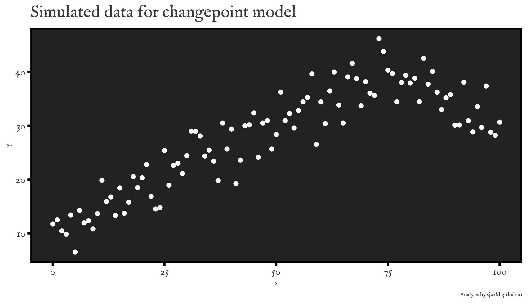
We’ll start by simulating some data that follows an increasing trend, then begins decreasing. As you can see from the plot below the code, there is a fairly clear breakpoint at 75, our true value.
alpha1 <- 10
alpha2 <- 60
beta1 <- .4
beta2 <- -.3
sigma <- 3
changepoint <- 75
set.seed(12345)
x <- seq(0, 100, by = 1)
y<- rep(0, N)

for(n in 1:length(x)){
  if(x[n] < changepoint){
    y[n] <- alpha1 + x[n] * beta1 + rnorm(1, 0, sigma)
  } else {
    y[n] <- alpha2 + x[n] * beta2 + rnorm(1, 0, sigma)
  }
}

# Plot data
ggplot(data.frame(x = x, y = y)) +
  geom_point(mapping = aes(x = x,
                           y = y),
             colour = "white") +
  labs(title = "Simulated data for changepoint model") +
  modified_theme_oppenheimer
ggsave("simulated_data_changepoint.png", width = 2000, height = 1150, units = "px")

Fitting the model
And with our simulated data, let’s fit our model. We’ll use weakly informative priors. As this is supposed to be a short blog post, we aren’t going to worry about prior predictive checks or anything else.
# Load changepoint model
changepoint_model <- cmdstan_model(paste0(here(), "/changepoint_model.stan"))

# Load data and fit model
stan_data_sim <- list(
  y = y,
  x = x,
  T = length(y),
  prior_alpha_sigma = 50,
  prior_beta_sigma = 10,
  prior_sigma = 2
)

fit_test <-  changepoint_model$sample(data = stan_data_sim,
                                      chains = 8,
                                      parallel_chains = 8,
                                      iter_warmup = 1000,
                                      iter_sampling = 2500)


# Plot draws
s_test <- as_draws_rvars(fit_test$draws("s"))
s_test %>%
  spread_draws(s) %>%
  ggplot(aes(x = s)) +
  stat_histinterval(colour = "grey65",
                    fill = "white") +
  labs(x = NULL,
       y = NULL,
       title = "Estimated changepoint",
       caption = "Analysis by sjwild.github.io") +
  modified_theme_oppenheimer +
  theme(axis.ticks.y = element_blank(),
        axis.text.y = element_blank())
ggsave("recovered_changepoint_simulated_data.png", width = 2000, height = 1150, units = "px")
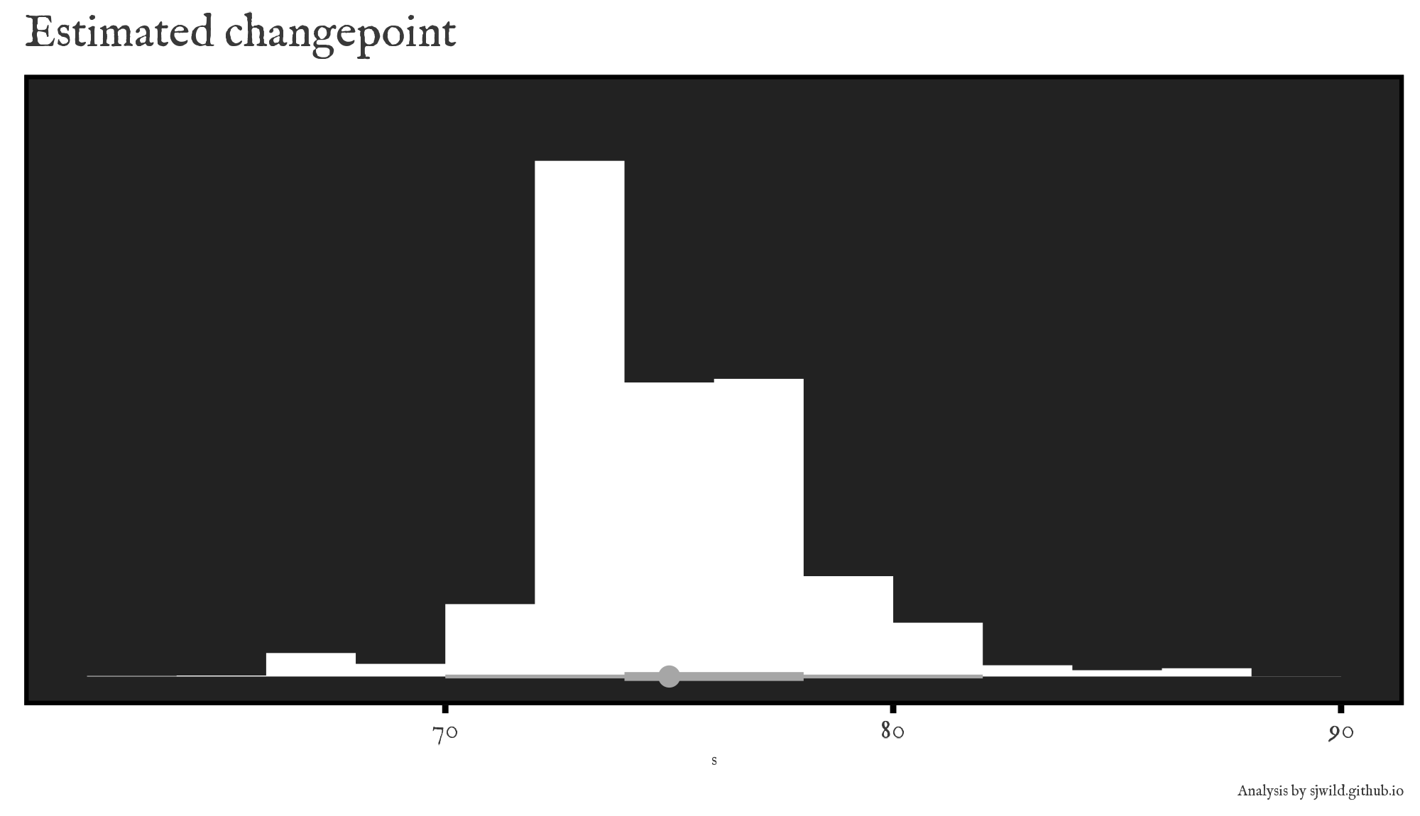
We get no warnings, so we’ll proceed. If this wasn’t a blog post, it would be worth doing the posterior predictive checks, testing other models and sensitivity to priors, etc. But this is good enough for us.

Fitting it to the Monitoring the Future data
Now that we know our model works, we’ll apply it to the Monitoring the Future. For simplicity, we’ll fit it to the global trend, rather than female and male trends.
d_agg_combined <- svyby(~Wk_out_cat, ~year, design = d_svy, FUN = svymean, na.rm = TRUE)
d_agg_combined$twice_or_more <- d_agg_combined$`Wk_out_cat2 or more times a week` * 100
d_agg_combined$se_twice_or_more <- d_agg_combined$`se.Wk_out_cat2 or more times a week` * 100

stan_data <- list(
  y = d_agg_combined$twice_or_more,
  x = d_agg_combined$year - min(d_agg_combined$year),
  T = nrow(d_agg_combined),
  prior_alpha_sigma = 50,
  prior_beta_sigma = 5,
  prior_sigma = 2
)


fit <- changepoint_model$sample(data = stan_data,
                                chains = 4,
                                parallel_chains = 4,
                                iter_warmup = 1000,
                                iter_sampling = 2000)


s <- as_draws_rvars(fit$draws("s"))
s %>%
  spread_draws(s) %>%
  mutate(s = s + min(d_agg_combined$year)) %>%
  ggplot(aes(x = s)) +
  stat_histinterval(colour = "grey65",
                    fill = "white") +
  labs(x = NULL,
       y = NULL,
       title = "Estimated changepoint in MTF data",
       caption = "Source: Monitoring the Future\nResponses to the question: During a typical week, on how many evenings do you go out for fun and recreation?
       Analysis by sjwild.github.io") +
  modified_theme_oppenheimer +
  theme(axis.ticks.y = element_blank(),
        axis.text.y = element_blank())
ggsave("recovered_changepoint_MTF.png", width = 2000, height = 1150, units = "px")

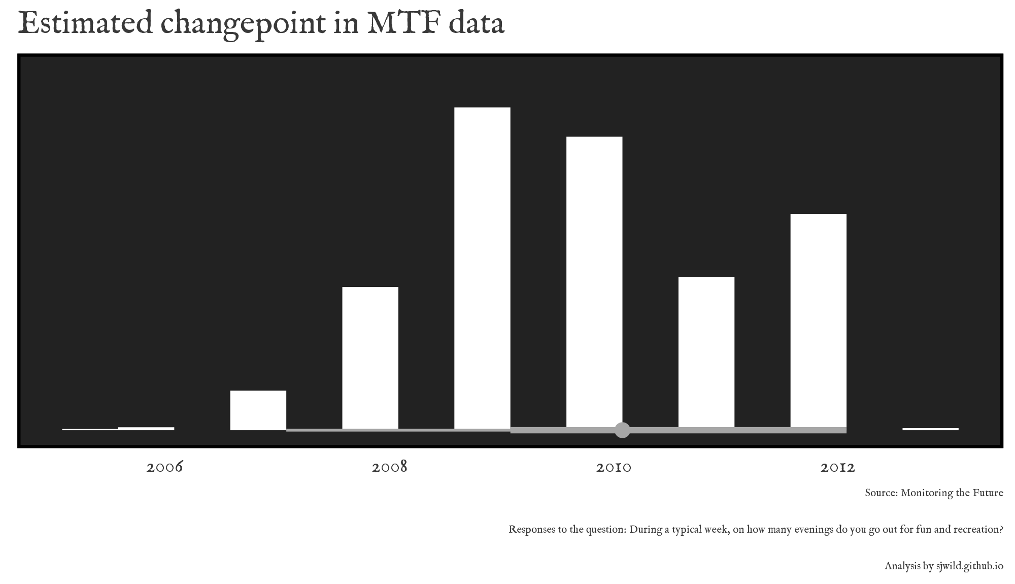
We can see that the mode is 2009, but it could easily be 2008 to 2012. But we imposed the assumption that there was only one changepoint. There oculd maybe be 2. If I was industrious, maybe I would fit another model. But that’s enough for today.
Sources
The data for Monitoring the Future can be download from here.
Here is the full list of studies, as requested in the docs for each study.
- Bachman, Jerald G., Johnston, Lloyd D., and O’Malley, Patrick M. Monitoring the Future: A Continuing Study of the Lifestyles and Values of Youth, 1976-1992: Concatenated Core File. Inter-university Consortium for Political and Social Research [distributor], 2008-11-24. https://doi.org/10.3886/ICPSR06227.v2
- Johnston, Lloyd D., Bachman, Jerald G., and O’Malley, Patrick M. Monitoring the Future: A Continuing Study of the Lifestyles and Values of Youth, 1993. Inter-university Consortium for Political and Social Research [distributor], 2006-08-21. https://doi.org/10.3886/ICPSR06367.v3
- Bachman, Jerald G., Johnston, Lloyd D., and O’Malley, Patrick M. Monitoring the Future: A Continuing Study of the Lifestyles and Values of Youth, 1994. Inter-university Consortium for Political and Social Research [distributor], 2007-06-29. https://doi.org/10.3886/ICPSR06517.v2
- Johnston, Lloyd D., Bachman, Jerald G., and O’Malley, Patrick M. Monitoring the Future: A Continuing Study of American Youth (12th-Grade Survey), 1995. Inter-university Consortium for Political and Social Research [distributor], 2007-09-07. https://doi.org/10.3886/ICPSR06716.v2
- Bachman, Jerald G., Johnston, Lloyd D., and O’Malley, Patrick M. Monitoring the Future: A Continuing Study of American Youth (12th-Grade Survey), 1996. Inter-university Consortium for Political and Social Research [distributor], 2005-11-04. https://doi.org/10.3886/ICPSR02268.v1
- Johnston, Lloyd D., Bachman, Jerald G., and O’Malley, Patrick M. Monitoring the Future: A Continuing Study of American Youth (12th-Grade Survey), 1997. Inter-university Consortium for Political and Social Research [distributor], 2006-05-15. https://doi.org/10.3886/ICPSR02477.v3
- Bachman, Jerald G., Johnston, Lloyd D., and O’Malley, Patrick M. Monitoring the Future: A Continuing Study of American Youth (12th-Grade Survey), 1998. Inter-university Consortium for Political and Social Research [distributor], 2006-05-15. https://doi.org/10.3886/ICPSR02751.v1
- Johnston, Lloyd D., Bachman, Jerald G., and O’Malley, Patrick M. Monitoring the Future: A Continuing Study of American Youth (12th-Grade Survey), 1999. Inter-university Consortium for Political and Social Research [distributor], 2007-09-18. https://doi.org/10.3886/ICPSR02939.v3
- Johnston, Lloyd D., Bachman, Jerald G., and O’Malley, Patrick M. Monitoring the Future: A Continuing Study of American Youth (12th-Grade Survey), 2000. Inter-university Consortium for Political and Social Research [distributor], 2006-05-15. https://doi.org/10.3886/ICPSR03184.v2
- Johnston, Lloyd D., Bachman, Jerald G., O’Malley, Patrick M., and Schulenberg, John E. Monitoring the Future: A Continuing Study of American Youth (12th-Grade Survey), 2001. Inter-university Consortium for Political and Social Research [distributor], 2006-05-16. https://doi.org/10.3886/ICPSR03425.v1
- Johnston, Lloyd D., Bachman, Jerald G., O’Malley, Patrick M., and Schulenberg, John E. Monitoring the Future: A Continuing Study of American Youth (12th-Grade Survey), 2002. Inter-university Consortium for Political and Social Research [distributor], 2006-05-15. https://doi.org/10.3886/ICPSR03753.v1
- Johnston, Lloyd D., Bachman, Jerald G., O’Malley, Patrick M., and Schulenberg, John E. Monitoring the Future: A Continuing Study of American Youth (12th-Grade Survey), 2003. Ann Arbor, MI: Inter-university Consortium for Political and Social Research [distributor], 2006-05-15. https://doi.org/10.3886/ICPSR04019.v1
- Johnston, Lloyd D., Bachman, Jerald G., O’Malley, Patrick M., and Schulenberg, John E. Monitoring the Future: A Continuing Study of American Youth (12th-Grade Survey), 2004. Inter-university Consortium for Political and Social Research [distributor], 2005-12-15. https://doi.org/10.3886/ICPSR04264.v1
- Johnston, Lloyd D., Bachman, Jerald G., O’Malley, Patrick M., and Schulenberg, John E. Monitoring the Future: A Continuing Study of American Youth (12th-Grade Survey), 2005. Inter-university Consortium for Political and Social Research [distributor], 2007-07-18. https://doi.org/10.3886/ICPSR04536.v3
- Johnston, Lloyd D., Bachman, Jerald G., O’Malley, Patrick M., and Schulenberg, John E. Monitoring the Future: A Continuing Study of American Youth (12th-Grade Survey), 2006. Inter-university Consortium for Political and Social Research [distributor], 2008-09-12. https://doi.org/10.3886/ICPSR20022.v3
- Johnston, Lloyd D., Bachman, Jerald G., O’Malley, Patrick M., and Schulenberg, John E. Monitoring the Future: A Continuing Study of American Youth (12th-Grade Survey), 2007. Inter-university Consortium for Political and Social Research [distributor], 2008-10-29. https://doi.org/10.3886/ICPSR22480.v1
- Johnston, Lloyd D., Bachman, Jerald G., O’Malley, Patrick M., and Schulenberg, John E. Monitoring the Future: A Continuing Study of American Youth (12th-Grade Survey), 2008. Inter-university Consortium for Political and Social Research [distributor], 2009-11-23. https://doi.org/10.3886/ICPSR25382.v2
- Johnston, Lloyd D., Bachman, Jerald G., O’Malley, Patrick M., and Schulenberg, John E. Monitoring the Future: A Continuing Study of American Youth (12th-Grade Survey), 2009. Inter-university Consortium for Political and Social Research [distributor], 2010-10-27. https://doi.org/10.3886/ICPSR28401.v1
- Johnston, Lloyd D., Bachman, Jerald G., O’Malley, Patrick M., and Schulenberg, John E. Monitoring the Future: A Continuing Study of American Youth (12th-Grade Survey), 2010. Inter-university Consortium for Political and Social Research [distributor], 2011-10-26. https://doi.org/10.3886/ICPSR30985.v1
- Johnston, Lloyd D., Bachman, Jerald G., O’Malley, Patrick M., and Schulenberg, John E. Monitoring the Future: A Continuing Study of American Youth (12th-Grade Survey), 2011. Inter-university Consortium for Political and Social Research [distributor], 2012-11-20. https://doi.org/10.3886/ICPSR34409.v2
- Johnston, Lloyd D., Bachman, Jerald G., O’Malley, Patrick M., and Schulenberg, John E. Monitoring the Future: A Continuing Study of American Youth (12th-Grade Survey), 2012. Inter-university Consortium for Political and Social Research [distributor], 2015-03-26. https://doi.org/10.3886/ICPSR34861.v3
- Johnston, Lloyd D., Bachman, Jerald G., O’Malley, Patrick M., and Schulenberg, John E. Monitoring the Future: A Continuing Study of American Youth (12th-Grade Survey), 2013. Inter-university Consortium for Political and Social Research [distributor], 2015-03-26. https://doi.org/10.3886/ICPSR35218.v2
- Johnston, Lloyd D., Bachman, Jerald G., O’Malley, Patrick M., Schulenberg, John E., and Miech, Richard A. Monitoring the Future: A Continuing Study of American Youth (12th-Grade Survey), 2014. Inter-university Consortium for Political and Social Research [distributor], 2017-05-24. https://doi.org/10.3886/ICPSR36263.v3
- Johnston, Lloyd D., Bachman, Jerald G., O’Malley, Patrick M., Schulenberg, John E., and Miech, Richard A. Monitoring the Future: A Continuing Study of American Youth (12th-Grade Survey), 2015. Inter-university Consortium for Political and Social Research [distributor], 2016-10-25. https://doi.org/10.3886/ICPSR36408.v1
- Johnston, Lloyd D., Bachman, Jerald G., O’Malley, Patrick M., Schulenberg, John E., and Miech, Richard A. Monitoring the Future: A Continuing Study of American Youth (12th-Grade Survey), 2016. Inter-university Consortium for Political and Social Research [distributor], 2017-10-26. https://doi.org/10.3886/ICPSR36798.v1
- Johnston, Lloyd D., Bachman, Jerald G., O’Malley, Patrick M., Schulenberg, John E., and Miech, Richard A. Monitoring the Future: A Continuing Study of American Youth (12th-Grade Survey), 2016. Inter-university Consortium for Political and Social Research [distributor], 2017-10-26. https://doi.org/10.3886/ICPSR36798.v1
- Miech, Richard A., Johnston, Lloyd D., Bachman, Jerald G., O’Malley, Patrick M., and Schulenberg, John E. Monitoring the Future: A Continuing Study of American Youth (12th-Grade Survey), 2017. Inter-university Consortium for Political and Social Research [distributor], 2018-10-29. https://doi.org/10.3886/ICPSR37182.v1
- Miech, Richard A., Johnston, Lloyd D., Bachman, Jerald G., O’Malley, Patrick M., and Schulenberg, John E. Monitoring the Future: A Continuing Study of American Youth (12th-Grade Survey), 2018. Inter-university Consortium for Political and Social Research [distributor], 2019-11-19. https://doi.org/10.3886/ICPSR37416.v1
- Miech, Richard A., Johnston, Lloyd D., Bachman, Jerald G., O’Malley, Patrick M., Schulenberg, John E., and Patrick, Megan E. Monitoring the Future: A Continuing Study of American Youth (12th-Grade Survey), 2019. Inter-university Consortium for Political and Social Research [distributor], 2020-10-29. https://doi.org/10.3886/ICPSR37841.v1
- Miech, Richard A., Johnston, Lloyd D., Bachman, Jerald G., O’Malley, Patrick M., Schulenberg, John E., and Patrick, Megan E. Monitoring the Future: A Continuing Study of American Youth (12th-Grade Survey), 2020. Inter-university Consortium for Political and Social Research [distributor], 2021-10-26. https://doi.org/10.3886/ICPSR38156.v1
- Miech, Richard A., Johnston, Lloyd D., Bachman, Jerald G., O’Malley, Patrick M., Schulenberg, John E., and Patrick, Megan E. Monitoring the Future: A Continuing Study of American Youth (12th-Grade Survey), 2021. Inter-university Consortium for Political and Social Research [distributor], 2022-10-31. https://doi.org/10.3886/ICPSR38503.v1
- Miech, Richard A., Johnston, Lloyd D., Bachman, Jerald G., O’Malley, Patrick M., Schulenberg, John E., and Patrick, Megan E. Monitoring the Future: A Continuing Study of American Youth (12th-Grade Survey), 2022. Inter-university Consortium for Political and Social Research [distributor], 2023-10-31. https://doi.org/10.3886/ICPSR38882.v1