Bayesian synthetic control using Julia and Stan
Synthetic control is a very popular causal inference technique. In synthetic control, we take a group of control units and weight them to produce a synthetic, or counterfactual, treated unit. In plain english, we take our control group and use it to pretend that our treated unit had never received the treatement.
How does synthetic control work? We take our control units and apply a set of weights to them under the idea that taking a little bit of each control unit lets us create a good fake treated unit. And there’s lots of merit to this idea.
But this blog post isn’t intended to get into the nitty-gritty of synthetic controls, nor is it intended to to be an intro to them. My assumption is that you already know what synthetic control is, or you are willing to read up on it for half an hour and then come back. There are a couple of great intros. Scott Cunningham’s The Mixtape and Nick Huntington-Klien’s The Effect both feature good, short intros to synthetic control. Those looking for a more detailed review can see Abadie’s Using Synthetic Control: Feasability, Data Requirements, and Methodological Aspects. Those who want to look at a few different ways of modelling synthetic control can check out Christopher P. Adams’ Learning Microeconometrics with R.
Some assumptions about you
Before we begin, I want to set out a few assumptions I have about you:
- You’re familiar with Julia, R, or some other programming language
- You’re familiar with Bayesian methods
- You’re familiar with Stan
- You’re interested in synthetic control
- You’re willing to put up with bad jokes, grammar, and spelling
Bayesian synthetic control
Most work on the theory of synthetic control or applying it tend use the frequentist version. But there is a Bayesian version too. At its heart, synthetic control is basically lasso or ridge regression to estimate the weights. We can use that idea to estimate a Bayesian version of synthetic control. There are few different versions floating around, including Broderson et al. (2015), Lee, Kim, and Gupta (2020), Pang, Liu, and Xu (2022), and Pinkney (2021).
Anyways, if you’ve read this far you obviously want to see some Bayesian synthetic control in action. So let’s go.
Showing that it works
To start with, we’re going to duplicate the example in The Mixtape. Cunningham was nice enough to include the code and data for his book, so we can duplicate the example in his book.
Let’s start by loading his data. While I’m using Julia and Stan for these examples, I will need to call on R to load the data. Unfortunately, the library Julia uses to open .dta files seems to have an error at the moment, and I cannot open .dta files with newer versions of Julia. Old versions work fine, but then I can’t use Stan. Compatability issues are awesome.
I’ve broken up the code to explain what I’m doing. If you just want the code, you can find it in the repo here.
# Load packages
ENV["CMDSTAN"] = expanduser("~/cmdstan/")
using Pkg

Pkg.activate("COVID_19")

using Plots, StatsPlots
using CSV, DataFrames, HTTP
using Dates, Measures
using Turing, ReverseDiff, Memoization
using StanSample
using RCall

# Note that ReadStatt.jl does not seem to work with Julia 1.7.2 yet.
# So we will use RCall
R"""
library(tidyverse)
library(haven)

# This code comes from Scot Cunningham's Mixtape
read_data <- function(df)
{
  full_path <- paste("https://raw.github.com/scunning1975/mixtape/master/",
                     df, sep = "")
  df <- read_dta(full_path)
  return(df)
}

texas <- read_data("texas.dta") %>%
  as.data.frame(.)

"""

df_texas = @rget texas
With that data, we are going to clean it and run our Stan model. We’re not going to fully duplicate Cunningham’s example here. He has the code in his book, so if you want to duplicate it you can get the code from there. We’re going to use code, however, to figure out which states to drop. The other change we are going to make is to drop the other predictors. We can always add them in later if we want.
drop_fips = [3, 7, 14, 43, 52] # States to drop


# Drop states
df_texas_bscm = df_texas[in(drop_fips).(df_texas.statefip) .== false, [:year, :statefip, :bmprison]]


# create name for state fips, which will be used as variable names when we go from long to widen format
df_texas_bscm.statefip = [join(["statefips_", df_texas_bscm.statefip[i]]) for i in 1:size(df_texas_bscm, 1)]
df_texas_bscm = unstack(df_texas_bscm, :statefip, :bmprison) # equivalent to pivot_wider


# build a vector and a matrix, than scale to help the sampler.
adj_factor = 10_000
ind = contains.(names(df_texas_bscm), "statefips_48") # index IDing texas
X_texas = Matrix{Float64}(df_texas_bscm[:, Not(ind)])[:, 2:51] ./ adj_factor
y_texas = Vector{Float64}(df_texas_bscm[:, ind][:, 1]) ./ adj_factor


# Matrices and vectors, divided into pre and post period
yr = 1993
X_texas_pre = X_texas[df_texas_bscm.year .≤ yr, :]
X_texas_post = X_texas[df_texas_bscm.year .> yr, :]
y_texas_pre = y_texas[df_texas_bscm.year .≤ yr]
y_texas_post = y_texas[df_texas_bscm.year .> yr]
In his book, Cunningham says that the policy change occurred in 1993. Given the length of time it takes to build prisons, it seems reasonable to include 1993 in our pre-treatment period. Even if the policy change was made in January 1993, we realistically wouldn’t see more prisons built for a couple of years.
With that, we are ready to run our model. In this case, I have chosen to use a modified version of the model used by Lee, Kim, and Gupta (2020). I have taken their original model and modified it so that uses the horshoe prior proposed in Piironen and Vehtari (2017). (As an added bonus, this is the version also used by brms). I found that the original code of Lee, Kim, and Gupta (2020) ran with divergent transitions when I applied it to Cunningham’s Texas example. The modified version runs without divergent transitions, at least for this example.
Here is the Stan code for our model.
data{

  // Dimensions
  int N_pre;                                // Number of observations in the pre-treatment periods
  int N_post;                               // Number of observations in the post-treatment periods
  int p;                                    // Number of predictors (control units)

  // scales
  real<lower=0> scale_alpha;               // prior std for the intercept
  real<lower=0> scale_g;                   // scale for the half-t prior for tau

  // slabs
  real<lower=0> slab_scale;                // slab scale for the regularized horseshoe
  real<lower=0> slab_df;                   // slab degrees of freedom for the regularized

  // nu for degrees of freedom
  real<lower=1> nu_g;                      // degrees of freedom for the half-t prior
  real<lower=1> nu_l;                      // degrees of freedom for the half-t priors

  // inputs
  matrix[N_pre, p] X_pre;                  // design matrix pre-treatment (no intercept)
  matrix[N_post, p] X_post;                // design matrix in the post-treatment period (no intercept)

  // y
  real y_pre[N_pre];                        // Treated unit in the pre-treatment periods

}

parameters{

  // alpha and beta
  real alpha;
  vector[p] beta_raw;                       // Control unit weights (will be transformed)

  // shrinkage parameters
  real<lower=0> tau;                        // Global shrinkage
  vector<lower=0>[p] lambda;                // Local shrinkage

  // sigma
  real logsigma;

  //other parameters
  real<lower=0> caux;

}

transformed parameters{

  // containers
  vector[p] beta;                                // Control unit weights
  vector<lower=0>[p] lambda_tilde;               // Local shrinkage
  vector[N_pre] mu;                              // y_hat in the pre-treatment period
  real<lower=0> sigma;                           // error term for regression
  real<lower=0> c;                               // slab scale


  // transformed parameters
  sigma = exp(logsigma);
  c = slab_scale * sqrt(caux);
  lambda_tilde = sqrt(square(c) * square(lambda) ./ (square(c) + square(tau) * square(lambda)));
  beta = beta_raw .* lambda_tilde * tau;
  mu = alpha + X_pre * beta;

}

model{

  // priors
  beta_raw ~ std_normal();
  lambda ~ student_t(nu_l, 0, 1);
  tau ~ student_t(nu_g, 0, scale_g * sigma);
  caux ~ inv_gamma(0.5 * slab_df, 0.5 * slab_df);
  alpha ~ normal(0, scale_alpha);

  // model
  y_pre ~ normal(mu, sigma);

}

generated quantities{
  //Post-treatment prediction & Log-likelihood
  vector[N_pre] y_fit;                        //Fitted synthetic control unit in the pre-treatment
  vector[N_post] y_post;                      //Predicted synthetic control unit in the post-treatment
  vector[N_pre] log_lik;                      //Log-likelihood
  for(f in 1:N_pre){
    y_fit[f] = normal_rng(alpha + X_pre[f,] * beta, sigma);
  }

  for(i in 1:N_post){
    y_post[i] = normal_rng(alpha + X_post[i,] * beta, sigma);
  }

  for (t in 1:N_pre){
    log_lik[t] = normal_lpdf(y_pre[t] | y_fit[t], sigma);
  }

}
With that, we will load our data into Stan and run the model. If the model is successful, then we will run the diagnostics and extract the parameters (if you want to see the weights) and generated quantities (for the estimated pre- and post-periods). There is lots of other model checking we should do, but are not going to do right now because this an already long blog post. And there’s still a lot to do.
# run stan model
# Note we need to transpose our X matrices
texas_data = Dict(

  "N_pre" => size(X_texas_pre', 2), # Numbers of pre observations
  "N_post" => size(X_texas_post', 2), # Number of post observations
  "p" => size(X_texas_pre', 1), # Size of donor pool
  "y_pre" => y_texas_pre,
  "X_pre" => X_texas_pre',
  "X_post" => X_texas_post',

  "scale_alpha" => 1,
  "scale_g" => 1,

  "slab_scale" => 1,
  "slab_df" => 5,

  "nu_g" => 3,
  "nu_l" => 3

)

# load temp directory for model output
tmpdir = joinpath(@__DIR__, "tmp")

# run model
sm = SampleModel("bscm", read("Stan/bscm_horseshoe_modified.stan", String), tmpdir)
rc_texas = stan_sample(sm;
                       data = texas_data,
                       num_samples = 1500,
                       num_warmups = 1500,
                       num_chains = 4,
                       delta = 0.999, # Micheal Betancourt is going to be so mad at me for this
                       max_depth = 15,
                       seed = 47318)

if success(rc_texas)
  diagnose(sm)
  params_out = DataFrame(read_samples(sm))
  gq = stan_generate_quantities(sm)
end
And with that, we can extract our data and plot it. We’re going to create two functions: The first one produces a base plot that we can modify later, the second function will summarize our predicted outcomes. We’ll be using these functions again, so it will save us repeating a bunch of code.
# Function to pull quantiles
function get_qs(y_pre_fit::DataFrame,
                y_est::DataFrame;
                ll::Float64 = 0.025,
                ul::Float64 = 0.975)

  fit_n = size(y_pre_fit, 2)
  est_n = size(y_est, 2)
  y_fit_m = [mean(y_pre_fit[:, i]) for i in 1:fit_n]
  y_fit_ll = [quantile(y_pre_fit[:, i], ll) for i in 1:fit_n]
  y_fit_ul = [quantile(y_pre_fit[:, i], ul) for i in 1:fit_n]

  # Next post period
  y_post_m = [mean(y_est[:, i]) for i in 1:est_n]
  y_post_ll = [quantile(y_est[:, i], ll) for i in 1:est_n]
  y_post_ul = [quantile(y_est[:, i], ul) for i in 1:est_n]

  # combine values into one vector each
  synth_m = vcat(y_fit_m, y_post_m)
  synth_ll = vcat(y_fit_ll, y_post_ll)
  synth_ul = vcat(y_fit_ul, y_post_ul)

  return synth_m, synth_ll, synth_ul

end

get_qs(y_pre_fit::Matrix{Float64}, y_est::Matrix{Float64}) = get_qs(DataFrame(y_pre_fit, :auto), DataFrame(y_est, :auto))


# Function to plot baseplot
function plot_base(title::String,
  ylabel::String,
  xlabel::String;
  title_position = :left,
  size = (800, 500),
  xrotation = 45,
  legend = :topleft,
  legend_foreground_color = nothing,
  bottom_margin = 17mm,
  left_margin = 5mm,
  tickfontsize = 12,
  titlefontsize = 16,
  legendfontsize = 10,
  guidefontsize = 14,
  grid = :off,
  kwargs...)

   return plot(;title = title,
    ylabel = ylabel,
    xlabel = xlabel,
    title_position = title_position,
    size = size,
    xrotation = xrotation,
    legend = legend,
    legend_foreground_color = legend_foreground_color,
    bottom_margin = bottom_margin, left_margin = left_margin,
    tickfontsize = tickfontsize, titlefontsize = titlefontsize,
    legendfontsize = legendfontsize,
    guidefontsize = guidefontsize,
    grid = grid, kwargs...)

end


# Plot outcome. Start by getting matrices of draws from pre- and post-treatment period
texas_fit = gq[:, 1:length(y_texas_pre)]
texas_est = gq[:, (length(y_texas_pre) + 1):(length(y_texas_pre) + length(y_texas_post))]
texas_m, texas_ll, texas_ul = get_qs(texas_fit, texas_est)


texas_trend = plot_base("Synthetic control estimates: Mixtape example of\nblack prison population in Texas",
                        "Number of black prisoners (10,000s)",
                        "Year";
                        top_margin = 5mm)
plot!(texas_trend, Int.(unique(df_texas.year)), texas_m,
      ribbon = (texas_m - texas_ll, texas_ul - texas_m),
      label = "Estimated trend",
      lw = 3,
      lc = :blue, fill = :blue)
plot!(texas_trend, Int.(unique(df_texas.year)), vcat(y_texas_pre, y_texas_post),
      label = "Actual",
      lc = :black,
      lw = 3);
vline!(texas_trend, [1993],
       lc = :blue, linestyle = :dash,
       linealpha = 0.5,
       label = "")
annotate!(texas_trend, 1992.9, 5.5,
          StatsPlots.text("Policy change",
          10, :right))
annotate!(texas_trend, 2000, -0.8,
          StatsPlots.text("Source: https://raw.github.com/scunning1975/mixtape/master/texas.dta
          Analysis by sjwild.github.io",
          :right, 7))
png(texas_trend, "Images/Texas/texas_synthetic_control_estimates")
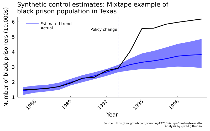
So our method works! Now we’re going to try it on something else: We’ll try estimate the effect of Alberta dropping most of its public health requirements to reduce the spread of COVID-19. To be clear, you should not in any way draw causal conclusion from what’s below.
Alberta public health measures
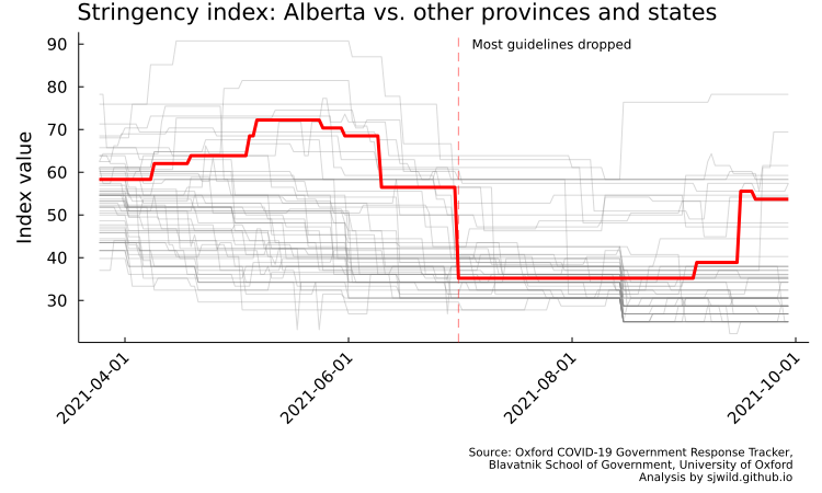
On July 1, 2021, Alberta reduced most of its public health requirements. As illustrated by the Oxford COVID-19 Government Response Tracker, Alberta went form being among the strictest provinces and states to being around the average (the code to produce the image below is in the repo).
Here is our research question: Did dropping most public health measures lead to more COVID-19 cases compared to an Alberta that had kept stricter public health measures? This gives our thoeretical and empirical estimand:
- Theoretical estimand: The difference in cumulative casses on day t between an Alberta that kept retrictions versus an Alberta that dropped its public health restrictions, that is \(\sum_{t=1}^T(Y_t(1) - Y_t(0))\)
- Target population: Alberta daily totals from July 1st, 2021 to September 30, 2021
- Empirical estimand: The difference in cumulative cases between observed Alberta and counterfactual Alberta from July 1st, 2021 to September 30, 2021, \(\sum_{t=1}^T(Y_t(\text{Alberta restrictions removed}) - Y_t(\text{Alberta restrictions maintained}))\)
And this, in turn, gives us our estimation strategy and outcome variable.
- Estimation strategy and outcome variable: We are going to use synthetic control to estimate log cumulative cases. Government reporting around COVID-19 cases varied by state or province, is filled with lots of corrections that aren’t necessarily reflected in a given day’s case count, is missing values because there is no reporting on certain days, etc. Cumulative cases help address some of these issues. It also has the added advantage of not being zero (generally), so we can take logs and estimate a log-log model. Caveat: If this were an academic article or a serious piece of modelling, I would probably use a different measure. But this is already a somewhat-long blog post, so this is our measure. Maybe in a future post.
Making a few assumptions explicit
In order to create our counterfactual Alberta, we need to make some assumptions. Here are a few I am going to make explicit, along with my (probably unjustifiable) reasons.
- Treatment date: July 1, 2021. Because of how COVID spreads, in this case it is reasonable to include July 1 in the post-treatment period. Overall, I don’t think it makes a difference which period July 1 is included in.
- Post-treatment period: Our post-treatment period will last 91 days, from July 1 until September 30, 2021. Alberta reintroduced public health measures starting on September 16, 2021. It takes a couple of weeks to see the effect of public health measures (based on my admittedly quick Google search. I could not find any good scholarly papers showing how long it takes for restrictions to have an effect), so I have a picked September 30 as somewhat arbitrary end date. Why September 30? Because it is the end of the month. There is nothing else special about it.
- Pre-treatment period: Our pre-treatment period will last from April 1 until June 30. As with September 30, there is nothing special about April 1, other than it is the start of the month. So this is also an arbitrary date.
- Strictness of measures: To build our donor pool, we are going to use any states or provinces that, on July 1, 2021, had an a greater stringency index based on the Oxford COVID-19 Government Response Tracker. In reality, by using this measure we’re practically ensuring that the exclusion restriction is violated. To make this measure work, we’re going to ignore measurement issues around “stringency” and assume that it is measuring something concrete, that it is correct, and that there are no other issues with it. There are lots of other measures we could use, so this one is somewhat arbitrary. Its advantage is that it covers both Canada and the US.
- Donor pool: COVID-19 public health measures varied in strictness by state or province. Some states and provinces were much more lax in some periods than others. Some followed a “let’er rip” strategy, while others were more cautious. So to build our counterfactual Alberta, we’re going to use those provinces or states who had “stricter” measures, at least acccording to the Oxford COVID-19 Government Response Tracker. We are also going to drop any states or provinces who record a bunch of zero cases in the pre-treatment period, because any weight times by zero is zero. A second reason for dropping zeros is that we are going to take the log of our outcome variable, and we can’t take the log of 0.
- Data sources: We are going to rely on data from Health Canada and the Center for Disease Control. This has the advantage of being data from a government source. The disadvantage is that other sources are pre-cleaned and may already address some of the issues above, but at the cost of some opaqueness around the methods used to clean it.
- Other predictors: At this point, we are not going to use other predictors. A better model would properly incorporate things like vaccination rates, demographic factors, an so on. But since this post is supposed to be a demonstration of Bayesian synthetic control, we are going to ignore those.
- No spillovers: We’re also going to assume that there are no spillovers, such as geographical spillover. That is, we are going to assume that what happens in Alberta stays in Alberta. People travel, so this an unrealistic assumption. But it works for this blog post.
Getting and cleaning our data
To estimate this effect, we are going to need to get the estimated cases per province and state. We’ll start by downloading our data from Health Canada and the CDC, then clean it slightly.
# Download data and prep it for later steps
# Load data for Canada
# ensure variable names are the same across Canada and US data
url_canada = "https://health-infobase.canada.ca/src/data/covidLive/covid19-download.csv"
df_canada = CSV.read(HTTP.get(url_canada).body, DataFrame)
rename!(df_canada, :prname => :Province_State,
                   :numtoday => :cases,
                   :numconf => :total_cases)
df_canada = df_canada[ in([1, 99]).(df_canada.pruid) .== false, :] # Keep only the provincial data


# Load data for US
url_cdc = "https://data.cdc.gov/api/views/9mfq-cb36/rows.csv?accessType=DOWNLOAD"
df_cdc = CSV.read(HTTP.get(url_cdc).body, DataFrame; normalizenames = true)
rename!(df_cdc, :submission_date => :date,
                :new_case => :cases,
                :tot_cases => :total_cases)
df_cdc.date = replace.(df_cdc.date, "/" => "-")
df_cdc.date = Date.(df_cdc.date, dateformat"mm-dd-yyyy")


# get full state names and combine with CDC data
state_url = "https://github.com/jasonong/List-of-US-States/raw/master/states.csv"
state_names = CSV.read(HTTP.get(state_url).body, DataFrame; normalizenames = true)
rename!(state_names, :Abbreviation => :state,
                     :State => :Province_State)
df_cdc = leftjoin(df_cdc, state_names, on = :state)
dropmissing!(df_cdc, :Province_State)


# Load stringency index
url_stringency = "https://github.com/OxCGRT/covid-policy-tracker/raw/master/data/OxCGRT_withnotes_2021.csv"
df_stringency = CSV.read(HTTP.get(url_stringency).body, DataFrame; normalizenames = true)
dropmissing!(df_stringency, :RegionName)
filter!(row -> in(["Canada", "United States"]).(row.CountryName), df_stringency)
df_stringency.Date = Date.(string.(df_stringency.Date), dateformat"yyyymmdd")


# build df and filter by date
df = append!(df_canada[:, [:date, :Province_State, :total_cases]], df_cdc[:, [:date, :Province_State, :total_cases]])
start_date = Date(2021, 07, 01) - Day(98)
end_date = Date(2021, 07, 01) + Day(90)
filter!(row -> start_date .≤ row.date .≤ end_date, df)


# add in population
# add in population totals to compute cases per 100k
# Data was download from websites of Statistics Canada and the US Census Bureau, then pre-cleaned to make it easier to use here
fn_usa = "Data/US population.csv"
fn_can = "Data/Canada population.csv"
pop_canada = CSV.read(fn_can, DataFrame; normalizenames = true,)
pop_usa = CSV.read(fn_usa, DataFrame; normalizenames = true,)
rename!(pop_usa, :State => :Province_State)
rename!(pop_canada, :Geography => :Province_State)
pop_canada.Province_State = replace.(pop_canada.Province_State, " 6" => "")


# clean and parse population
pop_canada.X2019 = replace.(pop_canada.X2019, "," => "")
pop_canada.X2019 = parse.(Float64, pop_canada.X2019)
pop_usa.X2019 = replace.(pop_usa.X2019, "," => "")
pop_usa.X2019 = parse.(Float64, pop_usa.X2019)
pop = append!(pop_canada[:, [:Province_State, :X2019]], pop_usa[:, [:Province_State, :X2019]])


# Produce plot showing cases per day and then showing seven-day moving average
# First, combine cases data and population data
# Then filter
date_list = unique(df.date)[2:end]
df.newdate = [join(["X", df.date[i]]) for i in 1:size(df, 1)]
df.newdate = replace.(df.newdate, "-" => "_")
df = unstack(df[:, [:newdate, :Province_State, :total_cases]], :newdate, :total_cases)
df = innerjoin(df, pop, on = :Province_State)
Fitting the first model to cumulative cases
First, we’re going to model cumulative cases. So we’ll extract our cumulative cases per day. Then we’ll normalize it so that different provinces and states are comparable. This is our empirical estimte, so we’re going to try model it directly.
We already have the model we tested on the Texas data, so we are going to use it because we know it works. In this particular case, we don’t need to use horseshoe priors, because we have fewer predictors than observations. I originally started modelling COVID cases using a shorter timeframe where horseshoe priors were necessary, but gradually lengthened the number of time periods while still using the same model.
We could also adjust the model, such as by using a lognormal likelihood. But we already used this model and it worked, so we are going to use it again. We’ll simply take \(ln(y)\) rather than use a lognormal likelihood. I leave using a different model (say a normal linear regression, or use a lognormal distribution) as an exercise to the reader. It’s trivial to modify the models. (Okay, bad math/stats jokes. I’m not sorry.)
In the code below, we are going to run our Stan model.
One important thing to note is that I have skipped a whole bunch of workflow steps, including prior predictive checks, starting with a simpler model and then building up, and so on. Likewise, I only run the Stan diagnostic bianaries. I don’t look at the traceplots, etc. You should always check these things. Don’t be like me here.
# to scale
pop_scale = 100_000


#total number of cases
y_direct = Matrix{Float64}(df[df.Province_State .== "Alberta", 9:(end-1)]) ./ df[df.Province_State .== "Alberta", end] * pop_scale
X_direct = Matrix{Float64}(df[df.Province_State .!= "Alberta", 9:(end-1)]) ./ df[df.Province_State .!= "Alberta", end] * pop_scale


# get names of all provinces and states that have a higher stringency on July 1,
# which is the date AB "opened for summer"
filter!(row -> row.Date .== Date(2021, 07, 01), df_stringency)
ab = df_stringency.StringencyIndex[df_stringency.RegionName .== "Alberta"]

# get value of AB stringecy index on July 1, 2021
stringency_idx = df_stringency.RegionName[df_stringency.StringencyIndex .> ab]

# Remove states with zero reported cases
indx = [sum(X_direct[i, :] .≤ 0) for i in 1:63]
X_direct = X_direct[indx .== 0, :]

# Get names of provinces and states with stringency
# index who are still in the dataset
Province_State = df.Province_State[df.Province_State .!= "Alberta"]
Province_State = Province_State[indx .== 0]

# Keep states and provinces with stringency index greater than AB
Province_State_idx = in(stringency_idx).(Province_State)


# Drop states with either excessive zeros or when stringency value is above thereshold
X_direct = X_direct[Province_State_idx, :]


# Log vales so we have a log-log model
y_direct = log.(y_direct)
X_direct = log.(X_direct)


# Fit normal model
# Build pre and post values
trt_value = 91
y_pre_direct = y_direct[1:trt_value]
y_post_direct = y_direct[(trt_value+1):end]
X_pre_direct = X_direct[:, 1:trt_value]
X_post_direct = X_direct[:, (trt_value+1):end]
y_mean_direct = y_pre_direct[end]
x_mean_direct = X_pre_direct[:, end]


# Remove means to centre values
y_pre_direct = (y_pre_direct .- y_mean_direct)
X_pre_direct = (X_pre_direct .- x_mean_direct)
y_post_direct = (y_post_direct .- y_mean_direct)
X_post_direct = (X_post_direct .- x_mean_direct)

AB_data_direct = Dict(

  "N_pre" => size(X_pre_direct, 2), # Numbers of pre observations
  "N_post" => size(X_post_direct, 2), # Number of post observations
  "p" => size(X_pre_direct, 1), # Size of donor pool
  "y_pre" => y_pre_direct,
  "X_pre" => X_pre_direct,
  "X_post" => X_post_direct,

  "scale_alpha" => 1,
  "scale_g" => 1,

  "slab_scale" => 1,
  "slab_df" => 5,

  "nu_g" => 3,
  "nu_l" => 3

)


# Run model
rc_AB_direct = stan_sample(sm;
                           data = AB_data_direct,
                           num_samples = 1000,
                           num_warmups = 1000,
                           num_chains = 4,
                           delta = 0.999,
                           max_depth = 20, # for some reason this was needed on an earlier version. Something is clearly wrong.
                           seed = 33294)


# check diagnostics and extract parameters
if success(rc_AB_direct)
    diagnose(sm)
    params_out = DataFrame(read_samples(sm))
    gq = stan_generate_quantities(sm)
end

y_fit_direct = gq[:, 1:length(y_pre_direct)] .+ y_mean_direct
y_post_est_direct = gq[:, (length(y_pre_direct) + 1):(length(y_pre_direct) + length(y_post_direct))] .+ y_mean_direct
y_fit_direct = exp.(y_fit_direct)
y_post_est_direct = exp.(y_post_est_direct)
AB_m_direct, AB_ll_direct, AB_ul_direct = get_qs(y_fit_direct, y_post_est_direct)

y_actual = Matrix{Float64}(df[df.Province_State .== "Alberta", 9:(end-1)]) ./ df[df.Province_State .== "Alberta", end] * pop_scale
y_actual = Vector(y_actual[1, :])

date_list = [(start_date + Day(7)):Day(1):end_date;]

# Plot directly modeled cumulative cases
AB_trend_direct = plot_base("Acutal vs estimated cases: Directly modelling\ncumulative cases",
                            "Num cases (per 100k)",
                            "Date")
plot!(AB_trend_direct, date_list, AB_m_direct,
      ribbon = (AB_m_direct - AB_ll_direct, AB_ul_direct - AB_m_direct),
      lc = :red, fill = :red, lw = 3,
      label = "Estimated trend";
      top_margin = 5mm)
plot!(AB_trend_direct, date_list, y_actual,
      label = "Actual",
      lc = :black,
      lw = 3)
vline!(AB_trend_direct, [Date(2021, 07, 01)],
       lc = :red, linestyle = :dash,
       linealpha = 0.5,
       label = "")
hline!(AB_trend_direct, [y_actual[91]],
       lc = :black, linestyle = :dash,
       linealpha = 0.5,
       lw = 2,
       label = "")
annotate!(AB_trend_direct, Date(2021, 07, 03), 8000,
          StatsPlots.text("Most guidelines dropped",
          10, :left))
annotate!(AB_trend_direct, Date(2021, 09, 30), 750,
          StatsPlots.text("Source: Government of Canada and CDC
          Analysis by sjwild.github.io",
          :right, 7))
png(AB_trend_direct, "Images/Alberta/directly_modelling_cumulative_cases")
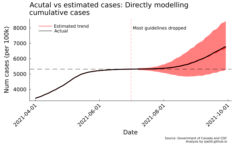
This model doesn’t work. While it converges, we can clearly see in the image above that it is making some inappropriate predictions: the lower bound of cumulative cases in the post-treatment period is predicted to fall below cumulative cases at the end of the pre-treatment period. That shouldn’t happen, because we can’t magically lose cases that already occured.
Building our second model
But if we think about how cumulative cases become cumulative cases, we can find another way to generate our empirical estimand. (But we don’t want to think too deeply. That might get us into SIER models, agent-based models, or something else. I know very little about some of those models. I leave trying them as an exercise to the reader.)
To get cumulative cases, we could also simply add up cases per day. We can do that here. To compute our daily cases, we’ll use the cumulative number of cases per day, minus the pervious day’s cumulative cases.
In the image below, you can see that a couple of states feature negative cases per day. This is a reporting artifact, where the state or province in question adjusted its total number of COVID cases. This could be because they changed who is counted as a COVID case, they accidentally over-reported, or other reasons. It’s impossible to have negative COVID cases per day, but we are going to leave it for now. To properly correct for the adjustments, we really need to do more research into the reason for adjustments and then decide how best to deal with it. So for now we are going to leave it as is.
Another issue you can see is that reporting “spikes” at regular intervals, then drops. This reflects daily testing trends. Weekends usually feature less testing than weekdays, so we see an increasing trend on weekdays, then drops over the weekend.
This is also a good reminder to always plot your data, otherwise it is easy to miss patterns like this.
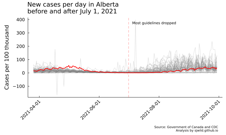
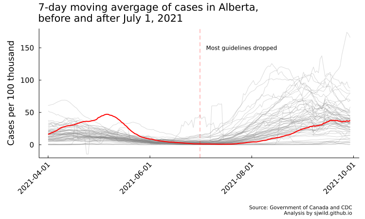
But how do the data look if we take the 7-day moving average? Pretty similar (code to compute the 7-day moving average and produce the plot is in the repo). We can still see the negative cases from the reporting adjustment, but they are less prominent here. We can also see that Alberta had a lot more cases in May than other provinces. This will be a good test to see if our model can reproduce that trend.
And with that, let’s fit our second model, this time using a 7-day moving average.
y = Vector{Float64}()
X = Matrix{Float64}(undef, (size(X_raw, 1), size(X_raw, 2) - 6))

# Calculate 7-day moving average
for j in 7:length(y_raw)
  push!(y, sum(y_raw[(j-6):j])/7)

  for i in 1:size(X_raw, 1)
    X[i, (j-6)] = sum(X_raw[i, (j-6):j]) / 7
  end

end


# Build indices to remove zero cases and states/provinces with lower stringency
indx = [sum(X[i, :] .≤ 0) for i in 1:63]
X = X[indx .== 0, :]
Province_State = df.Province_State[df.Province_State .!= "Alberta"]
Province_State = Province_State[indx .== 0]

# Keep states and provinces with stringency index greater than AB
Province_State_idx = in(stringency_idx).(Province_State)


# Subset X and build pre and post matrices
X = X[Province_State_idx, :]
y_pre = y[1:trt_value]
y_post = y[(trt_value+1):end]
X_pre = X[:, 1:trt_value]
X_post = X[:, (trt_value+1):end]

# Data for Stan
AB_data = Dict(

  "N_pre" => size(X_pre, 2), # Numbers of pre observations
  "N_post" => size(X_post, 2), # Number of post observations
  "p" => size(X_pre, 1), # Size of donor pool
  "y_pre" => log.(y_pre),
  "X_pre" => log.(X_pre),
  "X_post" => log.(X_post),

  "scale_alpha" => 1,
  "scale_g" => 1,

  "slab_scale" => 1,
  "slab_df" => 5,

  "nu_g" => 3,
  "nu_l" => 3

)


# Run model
rc_AB = stan_sample(sm;
                    data = AB_data,
                    num_samples = 1000,
                    num_warmups = 1000,
                    num_chains = 4,
                    delta = 0.999,
                    max_depth = 15,
                    seed = 33294)


# check diagnostics and extract parameters
if success(rc_AB)
    diagnose(sm)
    params_out = DataFrame(read_samples(sm))
    gq = stan_generate_quantities(sm)
end
Our model has finished running and the diagnostics look good. Now we’re ready to see how well it performed. With the code below we extract the estimated values, exponentiate them, and then summarize them. We’ll then plot the estimated trend and the true trend, and see what trend our counterfactual Alberta will follow.
# Transform parameters
y_fit = gq[:, 1:length(y_pre)]
y_post_est = gq[:, (length(y_pre) + 1):(length(y_pre) + length(y_post))]
y_fit = exp.(y_fit)
y_post_est = exp.(y_post_est)


# Build series for plotting.
# Start with pre-period fitted values
AB_m, AB_ll, AB_ul = get_qs(y_fit, y_post_est)

# dates
AB_trend = plot_base("Actual vs estimated cases using Alberta 7-day moving average",
                     "Num cases (per 100k)",
                     "Date";
                     legend = :bottomleft,
                     topmargin = 5mm)
plot!(date_list, AB_m,
      ribbon = (AB_m - AB_ll, AB_ul - AB_m),
      lc = :red, fill = :red, lw = 3,
      label = "Estimated trend")
plot!(AB_trend, date_list, vcat(y_pre, y_post),
      label = "Actual",
      lc = :black,
      lw = 3)
vline!(AB_trend, [Date(2021, 07, 01)],
       lc = :red, linestyle = :dash,
       linealpha = 0.5,
       label = "")
annotate!(AB_trend, Date(2021, 07, 03), 6500,
          StatsPlots.text("Most guidelines dropped",
          10, :left))
annotate!(AB_trend, Date(2021, 09, 30), -25,
          StatsPlots.text("Source: Government of Canada and CDC
          Analysis by sjwild.github.io",
          :right, 7))
png(AB_trend, "Images/Alberta/estimates_7_day_moving_average")
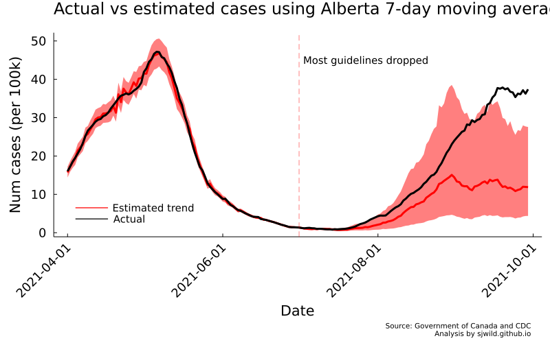
So there we have it. We can see that the pre-trend is pretty close. For the trend post-treatment, Alberta seems to get outside the 95% CI once September starts. That really doesn’t matter here, because we aren’t interested in the 7-day moving average itself. Instead, we are using it to compute cumulative cases, hopefully without our estimates giving us impossible values.
So let’s add the cases together to get our cumulative cases.
# Build counts by adding in values
cases_start = 3400.10

# Transform parameters and add
y_fit = gq[:, 1:length(y_pre)]
y_post_est = gq[:, (length(y_pre) + 1):(length(y_pre) + length(y_post))]
y_fit = exp.(y_fit)
y_post_est = exp.(y_post_est)
y_fit[:, 1] = y_fit[:, 1] .+ cases_start

for m in 2:size(y_fit, 2)
  for n in 1:size(y_fit, 1)
    y_fit[n, m] = sum(y_fit[n, (m-1):m])
  end
end

y_post_est[:, 1] = y_fit[:, end] + y_post_est[:, 1]

for m in 2:size(y_post_est, 2)
  for n in 1:size(y_post_est, 1)
    y_post_est[n, m] = sum(y_post_est[n, (m-1):m])
  end
end

# Build series for plotting.
# Start with pre-period fitted values
AB_m_c, AB_ll_c, AB_ul_c = get_qs(y_fit, y_post_est)


AB_trend_c = plot_base("Cumulative cases based on 7-day moving average",
                       "Num cases (per 100k)",
                       "Date";
                       legend = :topleft,
                       topmargin = 5mm)
plot!(AB_trend_c, date_list, AB_m_c,
      ribbon = (AB_m_c - AB_ll_c, AB_ul_c - AB_m_c),
      lc = :red, fill = :red, lw = 3,
      label = "Estimated trend")
plot!(AB_trend_c, date_list, y_actual,
      label = "Actual",
      lc = :black,
      lw = 3)
vline!(AB_trend_c, [Date(2021, 07, 01)],
       lc = :red, linestyle = :dash,
       linealpha = 0.5,
       label = "")
annotate!(AB_trend_c, Date(2021, 07, 03), 45,
          StatsPlots.text("Most guidelines dropped",
          10, :left))
annotate!(AB_trend_c, Date(2021, 09, 30), 1750,
          StatsPlots.text("Source: Government of Canada and CDC
          Analysis by sjwild.github.io",
          :right, 7))
png(AB_trend_c, "Images/Alberta/cumulative_cases_using_7_day_moving_average")
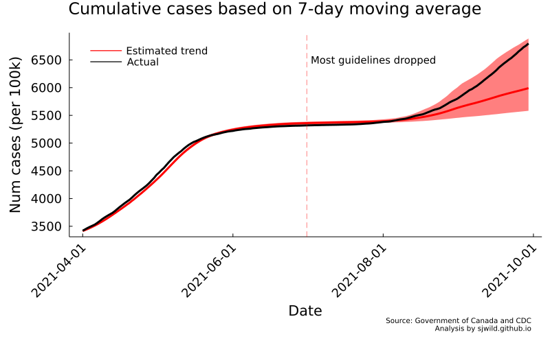
So what does this tell us? Assuming our model results in a good counterfactual Alberta (this is debateable, but let’s pretend it does), removing restrictions may have resulted in an increase of cases. But the actual observed cases are well within the 95% CIs for this model. Plus, if we take a close look, we can see that the model systematically underestimates then overestimates cases. Using the 7-day moving average is not a good choice here.
Let’s try modelling daily cases instead.
Third and final model for this post
This is our final model. For this one, we’ll try fit it to estimated daily cases. There’s going to be a few small changes when compared to the 7-day moving average model. First, we don’t want to drop any more donors from the donor pool. We’re therefore going to use the inverse hyberbolic sine function to transform our data. It’s used somewhat often to help address zero values in the data, and its inverse-link function is \(\frac{1}{2}e^y\). That makes it relatively easy to convert our values back to their original scale.
ihs(x) = log(x + sqrt(x^2 + 1))


# Subset data for modelling
X_raw = X_raw[indx .== 0, 7:end]
X_raw = X_raw[Province_State_idx, :]
y_raw = y_raw[7:end]


# Build pre and post values
y_pre_raw = y_raw[1:trt_value]
y_post_raw = y_raw[(trt_value+1):end]
X_pre_raw = X_raw[:, 1:trt_value]
X_post_raw = X_raw[:, (trt_value+1):end]

AB_data_ihs = Dict(

  "N_pre" => size(X_pre_raw, 2), # Numbers of pre observations
  "N_post" => size(X_post_raw, 2), # Number of post observations
  "p" => size(X_pre_raw, 1), # Size of donor pool
  "y_pre" => ihs.(y_pre_raw),
  "X_pre" => ihs.(X_pre_raw),
  "X_post" => ihs.(X_post_raw),

  "scale_alpha" => 1,
  "scale_g" => 1,

  "slab_scale" => 1,
  "slab_df" => 5,

  "nu_g" => 3,
  "nu_l" => 3

)

# run model
rc_ihs = stan_sample(sm;
                     data = AB_data_ihs,
                     num_samples = 1500,
                     num_warmups = 1500,
                     num_threads = 4,
                     delta = 0.999,
                     max_depth = 15,
                     seed = 21643)


if success(rc_ihs)
    diagnose(sm)
    params_out_ihs = DataFrame(read_samples(sm))
    gq_ihs = stan_generate_quantities(sm)
end

y_fit_ihs = exp.(gq_ihs[:, 1:length(y_pre_raw)]) ./ 2
y_post_est_ihs = exp.(gq_ihs[:, (length(y_pre_raw) + 1):(length(y_pre_raw) + length(y_post_raw))]) ./ 2
AB_m_ihs, AB_ll_ihs, AB_ul_ihs = get_qs(y_fit_ihs, y_post_est_ihs)


# Plot directly modeled cumulative cases
AB_trend_ihs = plot_base("Actual vs estimated daily COVID cases in Alberta",
                        "Num cases (per 100k)",
                        "Date";
                        ylims = (0, 90))
plot!(AB_trend_ihs, date_list, AB_m_ihs,
    ribbon = (AB_m_ihs - AB_ll_ihs, AB_ul_ihs - AB_m_ihs),
    lc = :red, fill = :red, lw = 3,
    label = "Estimated trend";
    top_margin = 5mm)
plot!(AB_trend_ihs, date_list, y_raw,
    label = "Actual",
    lc = :black,
    lw = 3)
vline!(AB_trend_ihs, [Date(2021, 07, 01)],
    lc = :red, linestyle = :dash,
    linealpha = 0.5,
    label = "")
annotate!(AB_trend_ihs, Date(2021, 07, 03), 80,
        StatsPlots.text("Most guidelines dropped",
        10, :left))
annotate!(AB_trend_ihs, Date(2021, 09, 30), -38,
          StatsPlots.text("Source: Government of Canada and CDC
          Analysis by sjwild.github.io",
          :right, 7))
png(AB_trend_ihs, "Images/Alberta/daily_cases_ihs")


# Now add in cases to get cumulative cases
y_fit_ihs[:, 1] = y_fit_ihs[:, 1] .+ cases_start
for m in 2:size(y_fit_ihs, 2)
    for n in 1:size(y_fit_ihs, 1)
      y_fit_ihs[n, m] = sum(y_fit_ihs[n, (m-1):m])
    end
end

y_post_est_ihs[:, 1] = y_fit_ihs[:, end] + y_post_est_ihs[:, 1]

for m in 2:size(y_post_est_ihs, 2)
    for n in 1:size(y_post_est_ihs, 1)
      y_post_est_ihs[n, m] = sum(y_post_est_ihs[n, (m-1):m])
    end
end


AB_m_ihs_c, AB_ll_ihs_c, AB_ul_ihs_c = get_qs(y_fit_ihs, y_post_est_ihs)


AB_trend_ihs_c = plot_base("Estimated vs actual cumulative cases in Alberta",
                           "Cumulative cases (per 100k)",
                           "Date";
                           legend = :topleft)
plot!(AB_trend_ihs_c, date_list, AB_m_ihs_c,
        ribbon = (AB_m_ihs_c - AB_ll_ihs_c, AB_ul_ihs_c - AB_m_ihs_c),
        lc = :red, fill = :red, lw = 3,
        label = "Estimated trend")
plot!(AB_trend_ihs_c, date_list, y_actual,
      label = "Actual",
      lc = :black,
      lw = 3)
vline!(AB_trend_ihs_c, [Date(2021, 07, 01)],
       lc = :red, linestyle = :dash,
       linealpha = 0.5,
       label = "")
annotate!(AB_trend_ihs_c, Date(2021, 07, 03), 6800,
            StatsPlots.text("Most guidelines dropped",
            10, :left))
annotate!(AB_trend_ihs_c, Date(2021, 09, 30), 1500,
            StatsPlots.text("Source: Government of Canada and CDC
            Analysis by sjwild.github.io",
            :right, 7))
png(AB_trend_ihs_c, "Images/Alberta/cumulative_cases_by_daily_cases")
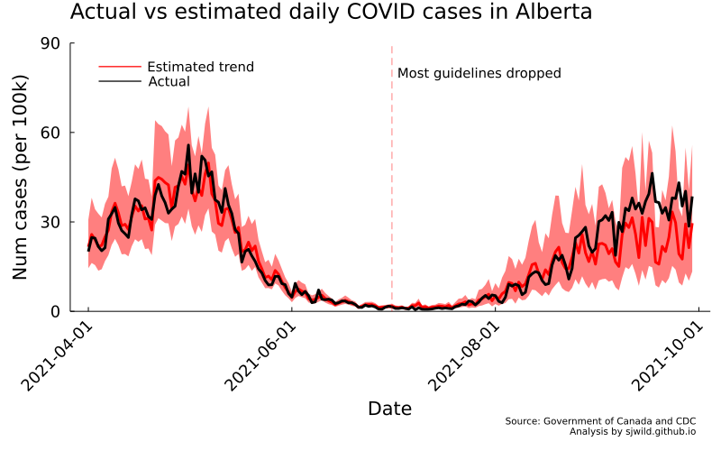
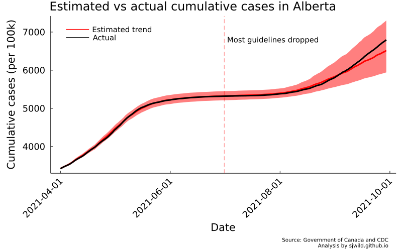
And there we go. We can see that the number of cases is slightly overestimated for some of the pre-treatment period. But overall, the trend looks pretty good. We can also see that the lower bound of estimates doesn’t fall below the lower bound for cases on June 30, 2021. In the post-treatment period, cumulative cases are well within the 95% CI. So the best we can say is that any effect of removing restrictions is too small for us to measure.
But wait, we wanted to know the difference in cases. So let’s do that before calling this post to a close.
y_cumulative = [y_fit_ihs y_post_est_ihs]
N, M = size(y_cumulative)
y_difference = Matrix{Float64}(undef, N, M)
for n in 1:N
    for m in 1:M
        y_difference[n, m] = y_actual[m] - y_cumulative[n, m]
    end
end


AB_m_d, AB_ll_d, AB_ul_d = get_qs(y_difference[:, 1:91], y_difference[:, 92:end])


AB_trend_d = plot_base("Difference in cases in Alberta",
                     "Difference (per 100k)",
                     "Date";
                     legend = :topleft)
plot!(AB_trend_d, date_list, AB_m_d,
        ribbon = (AB_m_d - AB_ll_d, AB_ul_d - AB_m_d),
        lc = :red, fill = :red, lw = 3,
        label = "Estimated trend")
vline!(AB_trend_d, [Date(2021, 07, 01)],
       lc = :red, linestyle = :dash,
       linealpha = 0.5,
       label = "")
hline!(AB_trend_d, [0],
       lc = :black, linestyle = :dash,
       linealpha = 0.5,
       lw = 2,
       label = "")
annotate!(AB_trend_d, Date(2021, 07, 03), 600,
            StatsPlots.text("Most guidelines dropped",
            10, :left))
annotate!(AB_trend_d, Date(2021, 09, 30), -1150,
            StatsPlots.text("Source: Government of Canada and CDC
            Analysis by sjwild.github.io",
            :right, 7))
png(AB_trend_d, "Images/Alberta/difference_in_cumulative_cases")
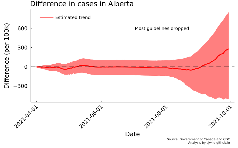
Looking at this image, we can clearly see that while there is a difference in cumulative cases, we cannot say for certain how large that difference was, or even if it was a positive or negative difference. While removing restrictions may have led to more cases, it is also plausible that it also led to fewer cases. The data is too noisy to say. So we should get better data.
Conclusion
With this post, we have seen how to estimate synthetic control models using Bayesian methods. Naturally, our model isn’t very good and there’s lots of ways to improve it: Maybe turning it into a state-space model, using SEIR models, adopting correlated errors, including other predictors, or building a better donor pool. You could try changing the likelihood, maybe even using a multivariate distribution to estimate several states or provinces simultaneously. But those are tasks for another post.